The world of AI and Machine Learning has many layers and can be quite complex to learn. Many terms are out there and unless you have a basic understanding of the landscape it can be quite confusing. In this article, expert Eric Enge will introduce the basic concepts and try to demystify it all for you. This is also the first of a four-part article series to cover many of the more interesting aspects of the AI landscape.
The other three articles in this series will be:
- Introduction to Natural Language Processing
- GPT-3: What It Is and How to Leverage It
- Current Google AI Algorithms: Rankbrain, BERT, MUM, and SMITH
Basic background on AI
There are so many different terms that it can be hard to sort out what they all mean. So let’s start with some definitions:
- Artificial Intelligence – This refers to intelligence possessed/demonstrated by machines, as opposed to natural intelligence, which is what we see in humans and other animals.
- Artificial General Intelligence (AGI) – This is a level of intelligence where machines are able to address any task that a human can. It does not exist yet, but many are striving to create it.
- Machine Learning – This is a subset of AI that uses data and iterative testing to learn how to perform specific tasks.
- Deep Learning – This is a subset of machine learning that leverages highly complex neural networks to solve more complex machine learning problems.
- Natural Language Processing (NLP) – This is the field of AI-focused specifically on processing and understanding language.
- Neural Networks – This is one of the more popular types of machine learning algorithms which attempts to model the way that neurons interact in the brain.
These are all closely related and it’s helpful to see how they all fit together:
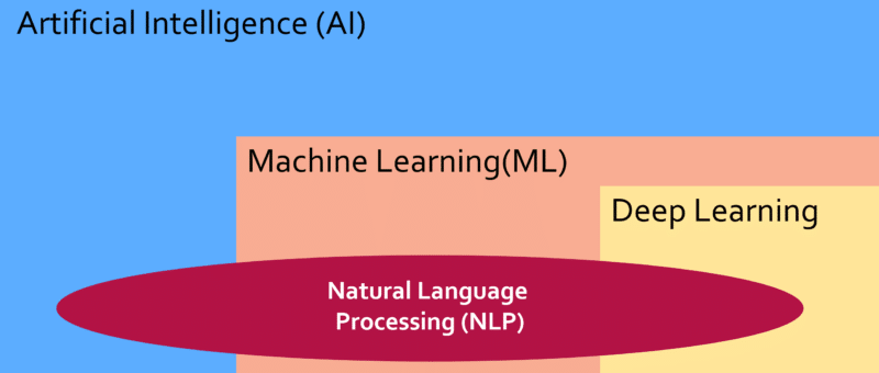
In summary, Artificial intelligence encompasses all of these concepts, deep learning is a subset of machine learning, and natural language processing uses a wide range of AI algorithms to better understand language.
Sample illustration of how a neural network works
There are many different types of machine learning algorithms. The most well-known of these are neural network algorithms and to provide you with a little context that’s what I’ll cover next.
Consider the problem of determining the salary for an employee. For example, what do we pay someone with 10 years of experience? To answer that question we can collect some data on what others are being paid and their years of experience, and that might look like this:
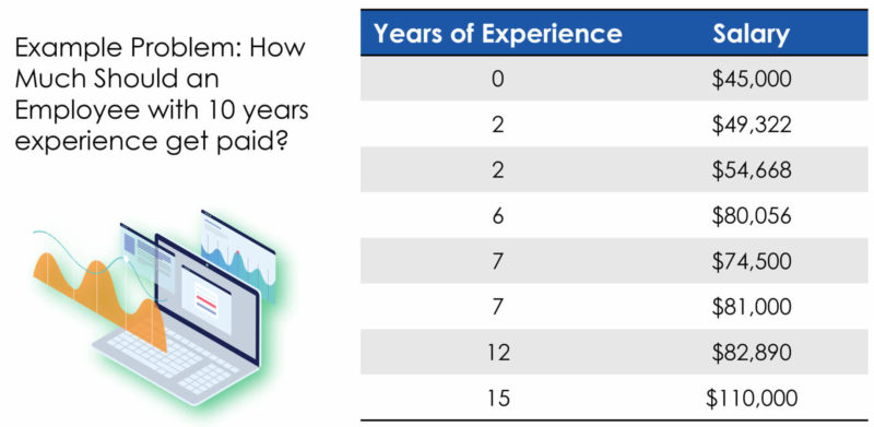
With data like this we can easily calculate what this particular employee should get paid by creating a line graph:

For this particular person, it suggests a salary of a little over $90,000 per year. However, we can all quickly recognize that this is not really a sufficient view as we also need to consider the nature of the job and the performance level of the employee. Introducing those two variables will lead us to a data chart more like this one:
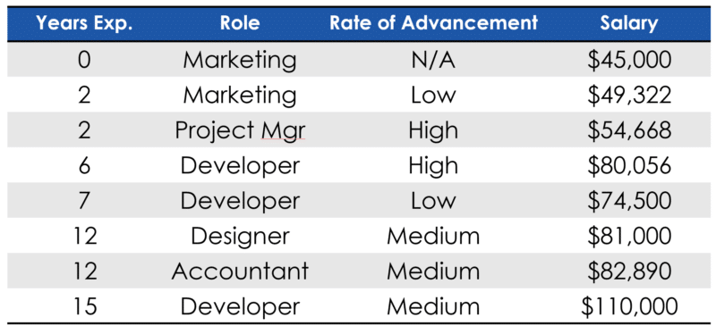
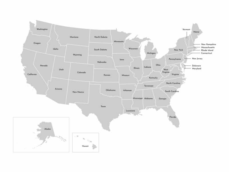
It’s a much tougher problem to solve but one that machine learning can do relatively easily. Yet, we’re not really done with adding complexity to the factors that impact salaries, as where you are located also has a large impact. For example, San Francisco Bay Area jobs in technology pay significantly more than the same jobs in many other parts of the country, in large part due to the large differences in the cost of living.
The basic approach that neural networks would use is to guess at the correct equation using the variables (job, years experience, performance level) and calculating the potential salary using that equation and seeing how well it matches our real-world data. This process is how neural networks are tuned and it is referred to as “gradient descent”. The simple English way to explain it would be to call it “successive approximation.”
The original salary data is what a neural network would use as “training data” so that it can know when it has built an algorithm that matches up with real-world experience. Let’s walk through a simple example starting with our original data set with just the years of experience and the salary data.
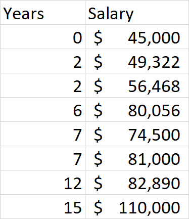
To keep our example simpler, let’s assume that the neural network that we’ll use for this understands that 0 years of experience equates to $45,000 in salary and that the basic form of the equation should be: Salary = Years of Service * X + $45,000. We need to work out the value of X to come up with the right equation to use. As a first step, the neural network might guess that the value of X is $1,500. In practice, these algorithms make these initial guesses randomly, but this will do for now. Here is what we get when we try a value of $1500:
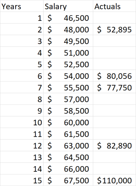
As we can see from the resulting data, the calculated values are too low. Neural networks are designed to compare the calculated values with the real values and provide that as feedback which can then be used to try a second guess at what the correct answer is. For our illustration, let’s have $3,000 be our next guess as the correct value for X. Here is what we get this time:
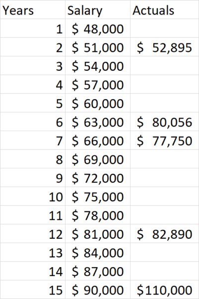
As we can see our results have improved, which is good! However, we still need to guess again because we’re not close enough to the right values. So, let’s try a guess of $6000 this time:
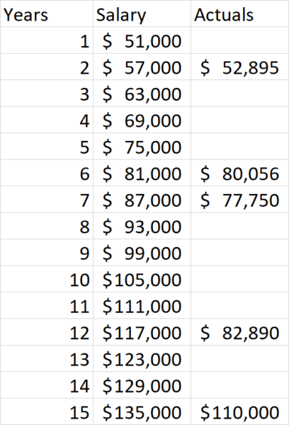
Interestingly, we now see that our margin of error has increased slightly, but we’re now too high! Perhaps we need to adjust our equations back down a bit. Let’s try $4500:
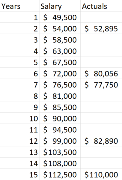
Now we see we’re quite close! We can keep trying additional values to see how much more we can improve the results. This brings into play another key value in machine learning which is how precise we want our algorithm to be and when do we stop iterating. But for purposes of our example here we’re close enough and hopefully you have an idea of how all this works.
Our example machine learning exercise had an extremely simple algorithm to build as we only needed to derive an equation in this form: Salary = Years of Service * X + $45,000 (aka y = mx + b). However, if we were trying to calculate a true salary algorithm that takes into all the factors that impact user salaries we would need:
- a much larger data set to use as our training data
- to build a much more complex algorithm
You can see how machine learning models can rapidly become highly complex. Imagine the complexities when we’re dealing with something on the scale of natural language processing!
Other types of basic machine learning algorithms
The machine learning example shared above is an example of what we call “supervised machine learning.” We call it supervised because we provided a training data set that contained target output values and the algorithm was able to use that to produce an equation that would generate the same (or close to the same) output results. There is also a class of machine learning algorithms that perform “unsupervised machine learning.”
With this class of algorithms, we still provide an input data set but don’t provide examples of the output data. The machine learning algorithms need to review the data and find meaning within the data on their own. This may sound scarily like human intelligence, but no, we’re not quite there yet. Let’s illustrate with two examples of this type of machine learning in the world.
One example of unsupervised machine learning is Google News. Google has the systems to discover articles getting the most traffic from hot new search queries that appear to be driven by new events. But how does it know that all the articles are on the same topic? While it can do traditional relevance matching the way they do in regular search in Google News this is done by algorithms that help them determine similarity between pieces of content.

As shown in the example image above, Google has successfully grouped numerous articles on the passage of the infrastructure bill on August 10th, 2021. As you might expect, each article that is focused on describing the event and the bill itself likely have substantial similarities in content. Recognizing these similarities and identifying articles is also an example of unsupervised machine learning in action.
Another interesting class of machine learning is what we call “recommender systems.” We see this in the real world on e-commerce sites like Amazon, or on movie sites like Netflix. On Amazon, we may see “Frequently Bought Together” underneath a listing on a product page. On other sites, this might be labeled something like “People who bought this also bought this.”
Movie sites like Netflix use similar systems to make movie recommendations to you. These might be based on specified preferences, movies you’ve rated, or your movie selection history. One popular approach to this is to compare the movies you’ve watched and rated highly with movies that have been watched and rated similarly by other users.
For example, if you’ve rated 4 action movies quite highly, and a different user (who we’ll call John) also rates action movies highly, the system might recommend to you other movies that John has watched but that you haven’t. This general approach is what is called “collaborative filtering” and is one of several approaches to building a recommender system.
Note: Thanks to Chris Penn for reviewing this article and providing guidance.
Opinions expressed in this article are those of the guest author and not necessarily Search Engine Land. Staff authors are listed here.

